Dynamic Scheduling for Flexible Manufactures

Author: Yuri Mauergauz

With the support of the MES center Russia and MES center ORG.

Abstract

Shop scheduling dynamics in total are caused by the current events in a shop during the prescribed plan period. Job sequence of the schedule essentially depends not only on the job processing time and the date but on the cost of machine adjusting, initial machine state, calendar of shop working days, presence of the staff, tool wear, calendar of machine maintenance, provision calendar for materials and other necessary resources.
Production scheduling in the paper embraces the set of twelve computer programs, which include similar algorithms. These algorithms are based on two general criteria simultaneously: the average order utility criterion, which is calculated by order utility functions, and the relative cost criterion of flexible manufacturing.

The order utility function is determined by the current production intensity of each order. All programs take into account the calendar of the shop working days, every program uses some of the restrictions enumerated above.
The programs of this set apply to the most of employed shop machine structures: single machines of different types; non-identical parallel machines which work either “make-to-stock” or “make-to-order”; flexible flow lines both in discrete and process manufacturing; shop floor scheduling; scheduling for industrial teams.
The software using the VBA language for MS Excel was designed, the examples of software applications are described. Necessary data is a set of records in MS Excel sheets. Results of scheduling are put down in sheets and forms both in text and in diagrams. Program texts are free to access.

Introduction

All possible quality criteria of the first SCOR (Supply Chain Operation Reference) model level relate to one of the four categories: customer service, economical indices, demand satisfaction flexibility, product development. The criteria of the last category are not usually considered in production planning, and demand satisfaction flexibility is ensured by strategy selection – “make-to-stock” or “make-to-order”. Therefore production planning quality mainly depends on the customer service level and production cost. The high customer service level (efficiency) may only be achieved through timely order completion. However, prompt order completion contradicts a high level of utilization and increases expenses. This trend is known as the dilemma of operation planning [Nyhuis and Wiendal, 2008]. Below we will examine some properties of industrial schedules, which are essentially important in the modern supply chain models.

Dynamic Scheduling

Dynamic of shop scheduling is caused by the total set of events realized in the industrial shop during a plan period. Let us enumerate such event’s kinds.

Receipt of a task with the job list for the directive plan horizon. The task includes estimated arrivals for pieces and materials. Jobs at the task usually are connected with customer orders, which are realized at the enterprise or may be concluded in the future.
Actual arrival of pieces and materials, which are provided by the task, into the shop.
Arrival of pieces and materials to the machine for processing.
Operation completion at the machine.
Processing order arrival, which is immediately supplied with pieces and materials.
Sudden events connected with breakage, staff absence, material spending and so on.

Among these events, only the task arrival and its data are strictly deterministic. Other events are either completely casual or having traits of casualness. Usually one out of two existing principles for shop scheduling is applied. At the first chance, the methods based on the job priority are used. At the second chance, there are different algorithms for scheduling with heuristic methods of decision search.

The plan task allows shop managers to elaborate a production schedule taking into account fulfillment of current jobs and plan dates for pieces and materials arrivals for new jobs. The notion “plan period” G is equal to some of working days. After the expiration of G, production schedule has to be calculated regularly. Such recalculation is obligatory to take account of accumulated changes in production situation, even when schedule is realized completely. In this paper, the plan period is recommended to be equal to a working week - usually 5 working days.

Existence of schedule does not determine its complete and suitable fulfillment, but it is extremely useful for industrial process preparing and organization. The schedule is calculated for a period, which is limited with plan horizon H in calendar hours. Plan horizon usually is equal or exceed plan period G. At the latter instance, the plan has be inevitably corrected. Correction also may be carried out at the every moment of plan execution owing to arising unforeseen circumstances.

Dynamic scheduling must be associated with the working calendar of the shop. It is necessary to kick-off the counting during scheduling from zero at the first plan calendar day. The commence moment of scheduling fulfillment here is equal to the moment of the first working day in format 18/09/2016 8:00 am. The shop plan staff usually works at the first (day) shift and elaborates or corrects the schedule for the next working day.

The scheduling calculation is always carried out with some accuracy. This paper recommends that owing to inaccuracy of initial data the time parameters have to be rounded off to 0.1 hour, or 6 minutes. So, value of 6 minutes is the time quantum during scheduling.

Quantity of working shifts is a main parameter of dynamic scheduling. Here it is supposed that the first shift begins at commencement of a working day, which is usually equal to 8 a.m. Duration of the working shift may be changed depending on industrial process. The most common duration is equal 8 hours, but it is not mandatory. When shop is loaded with work, two shifts both equal to 8 hours can used. If load is too big, or technology forbids interruptions, twenty-four-hour work may be applied. It may be the version of 3 shifts by 8 hours, or 2 shifts by 12 hours, or any other variant.

It is necessary to note that at twenty-four-hour work only the first shift applies to the current calendar day entirely. When a shop works with two shifts by 8 hours, the second shift finishes at the end of a calendar day too. However, if a shop works in 3 shifts by 8 hours, the last shift is working at the beginning of the next calendar day.

Sometimes it is necessary to take into account the possibility of duration changes in certain shifts. For instance, in pre-holiday or pre-rest day, the last shift (or even the single) shift may be shortened or cancelled. At the work day, which follows the rest day, commencement of the first shift usually coincides with the fixed commencement moment of the enterprise.

During a shift, the work interruptions may be introduced for food, sports or otherwise. As duration of such breaks is alike to original data accuracy, these breaks may be overlooked.

Flexible manufacturing

Flexible manufacturing facilitates to management of diverse changes at production surroundings. This manufacturing has some special properties:

objects of production must have accurate identification system;
manufacturing should be easy controlled by the planning and dispatching system;
quick readjustment of manufacturing should be implemented.

There are 7 kinds of flexibility: operation flexibility of the single machine; flexibility of manufacturing for various modifications of the produces; possibility for production output alternation; possibility for conversion to a new produce; flexibility of technological operation sequence; flexibility of the output value; service flexibility for the ready produces.

Flexibility of a certain machine using depends on duration of changeover, on complication of elaboration and input of computer program for operations, and, to considerable degree, on staff qualification. Peculiarities of machine design have great importance, which allowed various operations for produces of diverse sizes and volumes.

Necessity of manufacturing for various produce modifications is caused by the sparse of needs for various customers. In this case, production flexibility depends on the resources of production designers and managers, and on operational flexibility described above.

Alternation of production output of various kinds is essentially determined by production batch values. The lots and their sequence are the main task of production planning, and this paper is dedicated to such tasks.

Possibility for conversation to a new produce is generally and primarily estimated by economical point of view. Here, it is necessary to into account the means of production design, the equipment availability, assimilation difficulties and financial resources.

Flexibility of technological operation sequence exists when there is sufficient quantity of equipment, which is able to carry out the necessary technological operations. Besides, such equipment has to be provided with corresponding tools, materials and so on. When computer numerical control is used it has to be supplied with needed computer programs.

Change of the output value may be implemented when the conditions for sale are altered. There are some factors for such changes: equipment availability; sufficient staff number; financial resources of the enterprise. The problem of the output value may be not only the extension but diminution of volume. In such a case, the special arrangements are needed for staff and for equipment.

After production, the enterprise is often obliged to service the produced items. Flexibility here depends on cost of the special stations and working places for service, on personnel training, transportation, special apparatus and so on.

As a rule, it is impossible for an enterprise to achieve all kinds of flexibility simultaneously, so there is the problem of choice for the main aspects. When great flexibility is achieved, speed of production reaction on external influence essentially grows. In such a case, we have the agile manufacturing.

Group methods in scheduling

For the most types of manufacturing there are some problems listed below:

timely order fulfillment;
reduction of throughput time;
reduction of changeover time;
diminution of transportation cost;
sufficient equipment load;
even staff load;
increase of material using coefficient.

Let us to learn these questions in detail.

It is often assumed that the main task for a shop is to not frustrate the given due dates of manufactured objects for following treatment and assembling. In reality though, the enterprise management is usually aimed at tardiness revealing, and after this, to applying certain corrective actions over such contractors. In the same time, manufacturing before the due date is never controlled. However, in such a case the manufactured objects are kept in a warehouse for a long time, and this fact furthers immobilization of working capital and cluttering of a shop. Therefore we have to strive not only for attainment of due dates, but to make pieces, parts and assemblies at the moments near due dates. This method is known as Just-in-Time, which proved really useful in large-scale production.

Reduction of the throughput time depends on the decrease in the pre-processing time and transport time during manufacturing. Issues listed as c) and d) are caused by aspiration to diminish labor costs on processing and transportation. When these costs increase, the manufacturing duration, the throughput time and the total cost increase too. Said labor costs are spent on the each technological or transfer batch, so decreasing of batch number costs to go down.

In many cases, especially when the new expensive equipment is applied, enterprise managers strive to increase the machine load to pay the expenses. Of course, any equipment may not be loaded by 100%, but there are such attempts sometimes. It is reasonable to follow the policy to load the equipment sufficiently (70-80 %), allowing for time intervals for the working task corrections and for the systematic maintenance.

Regards for staff during manufacturing has great influence over shop work. It is necessary to take into account the natural wishes of workers for the high and stable wages, even engagement over a week and a working day and to avoid the tiredness caused by prolonged monotonous work. Unfortunately, an enterprise working at the market is subjected to demand variations for its production, and this factor inevitably leads to changes of staff quantity.

The result of any production is not only ready produces, but waste too. Of course, waste amount has to be as low as it is possible. For instance, the rational cut cards may be used. However, if the production plans change often and abruptly, the cards elaborated beforehand quickly become outdated.

As a result, we must note that majority of the issues identified, namely b), c), d), e), g), are economical in nature, i.e. production costs. Indeed, increase of labor amount in b), c), d) immediately entails to wages increase; insufficient equipment load in e) entails to depreciation costs increase; taste in g) entails to material costs increase.

At the same time, need for timely order completion in a) cannot be reduced to the costs only. Any attempts for so-called “penalty for delay” in scheduling are subjective and, as a rule, do not correspond to the current reality. The issue in f) is of social and psychological kind and cannot be reduced nor to economic or any other aspects.

Moving to the methods to solve said issues we must note that timely order completion, which provides the high efficiency rate, may be attained usually at the expense of batch diminution. However, this way contradicts to request of low production costs. Aspiration for improvement of these two indices simultaneously is “dilemma of planning” mentioned above.

As improvement of the cost criteria indices always makes the efficiency criteria go down, we, as a rule, cannot receive the single solution by optimization methods. Therefore, computing can only achieve the set of non-dominated (Pareto) solutions, and the user has to make the final decision. For this aim it is convenient to use the decision support systems, which are able to simulate scheduling at various input parameters and to find most suitable version for the current situation.

The main method for described tasks solution is the group planning. It includes calculation of rational production batches and elaboration of plans and schedules. Size of lots and their sequence are essentially depends on order volumes and due dates. This connection may be briefly formulated as: manufacturing is made by batches, but shipping is made by orders.

The group planning is the natural development of the group industrial technology. The latter one is the conception of production and organisation which uses likeness of construction and technologic parameters of various objects. The grouping is made when similar objects are found in the set. The similar objects are joined into the families, and within the family objects are classified by various traits. The lowest level, the family division always ends with an object type: this is a set of objects in a family, which has very near technological parameters in current manufacturing.

Group technology allows considerable possibility in decreasing of changeover time and cost. However, it is not always realized. The degree of group technology using is defined by perfection of the current calendar planning.

Attempts for group technology were made during the last 80 years, and they resulted in successful production when manufacturing was stable. However, in the last decades there are quick changes within all fields of human activity, and in production activity too. Therefore, grouping of working tasks now may only be effective if it is made on-line or just moments before the manufacturing starts.

Now, at each planning on any level there is a new set of working tasks. Therefore, technology grouping demands to calculate a corresponding plan quickly, and it is now possible owing to computers accession. The most simple plan grouping may be designed for types of objects, for example, on the construction designations. In particular, when the production plan is elaborated for some part batches with designations distinguished by versions these batches may be associated with the common type and possibly grouped.

Group planning may be carried out on the inter-shop level and on the intra-shop level. This paper shall cover scheduling inside the shop only. For this aim dynamic schedules are elaborated with two criteria simultaneously: the first criterion is the timely order completion, the second criterion is the costs of processing and changeovers.

The remainder of this paper is organized as follows. Section 2 provides order parameters the paper is based on. Section 3 determines the scheduling tree. Section 4 describes criteria for cutting of non-perspective branches. Section 5 formulates the standard scheduling algorithm. Section 6 is dedicated to brief description of the designed computer programs. In Section 7 some program examples are described. Section 8 contains some concluding remarks.

The order properties determining the industrial schedule

A set of batches in the schedule and their sequence primarily depend on numeral parameters of jobs in a working task. For simplicity, let us assume that jobs in a task are coincided with customer orders. In this case, each order has two main parameters for scheduling: a) directive due date in calendar days or hours and b) processing time in hours. Below two notions, which were proposed by author, are described for each order and are essentially applied in the paper.

Production Intensity

When criteria for an optimal plan to be performed are determined, in addition to process or economic factors, we also should take account of personal relations between responsible persons. There are two key courses of decision making i.e.: rational and psychological. As for the rational course, decisions are based on mathematically proven results while psychological course of decision making is substantially based on intuition and psychology of employees. A good production plan should be well-balanced between needs and wishes of all people involved into the production process.

People involved into the production process are all part of an extensive network of relations that can be considered as a certain psychological field. Each field, e.g., magnetic or electric has a quantitative characteristic that is called “intensity”. Similarly, a psychological field arising during production process can also be described quantitatively; this quantitative description is called the production intensity H [Mauergauz, 1999]. However, unlike physical fields, production intensity cannot be measured physically; it has no physical dimensions i.e. it is a dimensionless value.

Such dimensionless intensity of a psychological field (whether large or small) can only be estimated by comparison with another field or with another state of this field, e.g., at any other point of time. We face a natural question: how to calculate production intensity?

For the purpose of intensity quantification, let us take note of the fact that the situation in a production shop is mainly characterized by two factors i.e.: total time required for job completion and slack time. Please remember the so called dynamic priority rules described above that take account of these two factors. These rules include the Minimum Slack Time (MST), Critical Ratio (CR), and the Apparent Tardiness Cost (ATC) rules.

However, criteria calculated under any of these rules have substantial deficiencies. First, there is no way to determine the values of such criteria if the job due date has already expired by the start of planning. However, the most important thing is that the cumulative machine and personnel load resulting from different jobs cannot be determined using such criteria.

Unlike the above dynamic priority rules, we can determine production intensity values not only for each job, but for each machine and for the production shop overall. Production intensity for a certain machine will equal the sum of intensities for jobs awaiting processing on such machine; while production intensity for a production shop overall equals the sum of intensities for all jobs or, which is the same, for all machines.

The total time required to perform “top-to-bottom” plan targets is made of two values i.e. the production processing time, transfer time and changeover time. Slack time can be a positive or negative value or be equal to zero. Therefore, calculation relations used to determine production intensity should be different at different signs of slack time values.

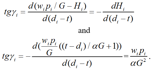
Thus, for one i-job:

(1)

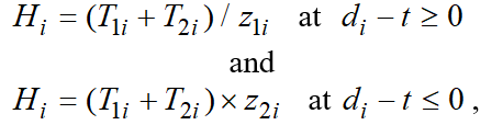
Where is the time duration determined by processing time pending at the time of planning; is the time component arising from the need to transfer jobs for further processing; is the production slack time in relation to plan targets; and is the tardiness from working task.

can be determined based on the following relation:

(2)

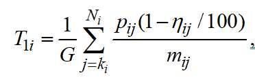
Where is the number of the first unfinished j-operation for i-job; is the total number of operations required to perform i-job; is the processing time of each remaining operation in hours or days; is the coefficient of readiness of j-operation (%); is the number of simultaneously processed items of i-job during j-operation; and is the average number of work hours or days in a planning period.

is calculated using the following relation:

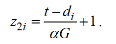
(3)

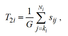
Where is the duration of required transportation and machine setup associated with j- operation for i-job.

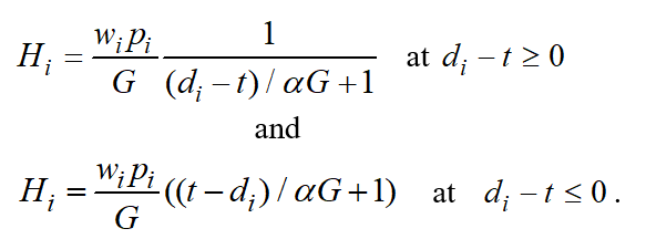
Let's assume the following relation for dimensionless slack time available to a planning engineer:

(4)

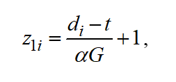
Where is the “psychological” coefficient of a given enterprise representing the level of "complacency” at available slack times or the level of “nervousness” if production due dates are failed to meet.

And, finally:

(5)

Similarly to the WSPT or ATC rules described above, intensity of a certain job can include a respective weight coefficient of priority . In particular, in the simplest case (where all readiness coefficients =0, the number of simultaneously processed items under one job =1, planning takes place for the first operation and all =1, while transportation and setup time can be ignored) intensity can be determined using the following formulas:

(6)

Now let’s consider the relation between intensity and available slack time or deadline tardiness (Figure 1).

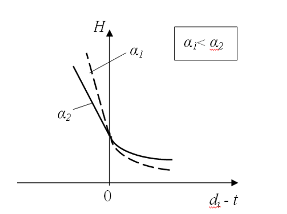
Figure 1. The relation between production intensity and slack time.

The slack time (difference between the due date for each job and the current time point ) is plotted on the X-line. On the positive part i.e. where , intensity values decrease hyperbolically as far as slack time increases. If slack time is negative i.e. there are tardiness on plan targets , intensity values increase linearly as far as tardiness increases. In expressions (4) and (5) if i.e. at the point of transfer from one relation to another, . Intensity values calculated using formulas (4) or (5) also coincide at this point. Besides, this point also sees the match of values for the following derivative:

6.5

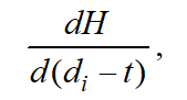
which have been calculated been using both formulas. Thus, the straight line in the left-hand part of the chart is tangent at the transition point to the hyperbolic curve in the right-hand part of the chart.

Production intensity is dimensionless and has not any physical sense, but it has “psychological” sense. Really, increasing of production intensity grows anxiety for order completion. Figure 1 shows two curves for H changes; these curves differ by the value of “psychological” coefficient ; note that . As we can see, the greater is, the less intensity is associated with tardiness; however, the level of “relaxation” is also lower when slack time is available.

Dynamic utility function of order

We can use functions of the dynamic utility of orders V to evaluate whether it is possible and desirable to ensure a high level of customer service. Let’s assume that any order is quite useful for a manufacturer in a certain prospect. Note that the greater the order scope and order completion time is, the greater utility such order will have. In such a way, the possibility of order completion in future certainly has a positive utility and should yield a respective gain.

On the other hand, the closer the due date for an order is, a manufacturer starts facing certain difficulties. The utility value starts decreasing. However, if the manufacturer manages to perform the order when due, the order utility remains positive till the very time of order execution; and utility becomes zero at the time of completion. If the manufacturer fails to meet the due date, he usually gets into troubles with this. The order becomes the source of losses, thus, having a negative utility.

As we can see, if slack time is available for an order, a manufacturer generally counts on gain while in case of tardiness it incurs losses. The behavior of utility as a potential gain/loss function is described in numerous sources. Generally, all research results can be reduced to two options shown in Figure 2 [Mauergauz, 2016].

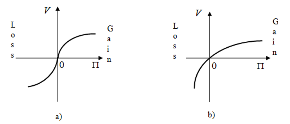
Figure 2. Charts of utility: potential gain/loss.

The gain value is plotted on the X-line (potential gain); the gain utility is plotted on the Y-line in the positive part of the X-line and the loss utility is plotted on the Y-line in the negative part of the X-line. The curve in Figure 2.a has been known as S-curve after well-know research of [Kahneman and Tversky,1984] that were awarded the Nobel Prize in the field of economics in 2002. Their research proved that people usually tend to take risks if there is a probability of potential loss (left-hand part of the chart in Figure 2.a). In this case, the concave left-hand part of the curve represents negative risk aversion - the second derivative has a positive sign at this interval of 2.a curve.

Unlike 2.a curve, 2.b curve always has a positive risk aversion no matter whether there is a probability of gain or loss. Please note that the chart of 2.b type [Grayson, 1960] was developed much earlier that 2.a chart. Differences between 2.а and 2.b curves probably arise from the pools of respondents and areas of money allocations. Studies Figure 2.a featured polls with low-income respondents whose income were insignificants and mainly used for personal consumption while studies in Figure 2.a dealt with large corporate investments.

Let’s use the above results of economic and psychological studies in order to build a function of dynamic utility of orders. Let’s assume that the current utility of i-order is as follows:

(7)

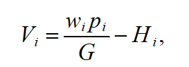
Where (as before) represents the processing time in days (hours) that remains before job completion; is the weight coefficient of priority; is slack time in days (hours) during the planning period; and is the production intensity associated with the order (job).

Let’s see how the dynamic utility function depends on slack time available till the established order due date (Figure 3) assuming that the orders has not yet been started i.e. does not depend on time.

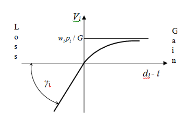
Figure 3. Dynamic order utility curve.

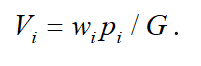
The depicted curve in the positive part of Figure 3 ( ) approaches the asymptote.

(8)

In the negative part ( ) the curve gets transformed into a straight line for which:

(9)

If we compare the curve in Figure 3 with the curves in Figure 2, we can see that the slack time available for a job determines gain or loss on Figure 3. The presence of an order is a substantial gain in a far prospect but the rate of gain growth decreases with the farness. In this part the behavior of the order utility function curve is absolutely similar to both curves shown in Figure 2.

The negative part of Figure 3 is similar to the loss part in Figure 2. In this part the curves in Figure 2 have different shapes. In order to check if the curve in Figure 3 is correct in the negative part, let’s assume human behavior as described above. As corporate managers use dynamic utility functions, their behaviour will be closer to the curve in Figure 2.b rather than 2.a curve as they are unlikely to take risks even in the loss part.

However, this is formally impossible to use 2.b curve as the order utility function as positive risk aversion typical of this curve results in a sharp increase of negative utility and, consequently, limits the potential loss value. The order utility function shall not have such a limit as, actually, any tardiness is possible during order execution. Therefore, the correct behavior will be a linear drop of the dynamic order utility function where risk aversion (the second derivative of the function) equals to zero. Figure 3 shows exactly this dependency.

Due to its additivity properties, both the production intensity and order utility for different orders can be added. Therefore, the average utility of the whole set of orders can be calculated.

If the number of order is at the planning horizon, their cumulative utility equals to the sum of utilities of each order as orders are generally independent. Orders, as a rule, are independent and the total value of the function of the current utility of orders:

(10)

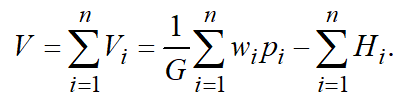
Value of function changes in time as the slack time available for a job is alternating. Besides, some orders are completed, and new orders arrive.

Design of the scheduling solutions tree

The solution tree is the outlined presentation for a scheduling decision issue. The branches of the tree are various events (solutions), and the nodes are key states where a decision is needed. Usually, the tree of solution is designed top-to-bottom, starting from the root. Figure 4 depicts the tree scheduling layout. Here the apices (nodes) are designated by circles and the branches are half-lines, which come from nodes of some level to nodes of next level. Nodes of the last level are named as leaves.

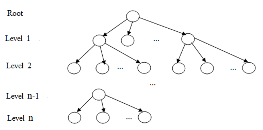Figure 4. Tree of scheduling solutions.

Any branch of the solution tree represents the event with a single job (or operation), which is carried out on a certain machine. In the node, all needed parameters are recorded: used fixtures; time of processing fulfillment; possible job volume and so on.

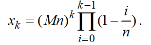
Let is assume the number of jobs, which is planned for horizon h, is equal to n, and each job may be realized on each machine of a set M. Then the number of half-lines from the root (level 1) is

(11)

Generally, on the next level, the number of planned jobs decreases by one:

(12)

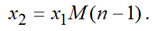
Following this process, we have on level

(13)

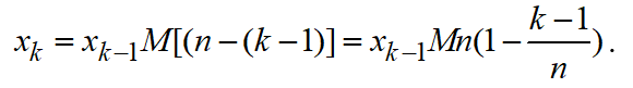
Mathematical relation (13) is geometrical progression with alternating denominator. There is distinction from usual geometric progression with constant denominator — the multiplier, which depends on a number of member in geometrical progression. Using formulas (11-13), for member in geometrical progression,

(14)

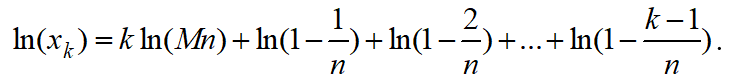
According to (14), the quantity of nodes with increasing level number in the beginning grows quickly, but owing to the multiplier of product type, after some moment the quantity diminishes. Let us find the level with maximum of node quantity. Logarithm for (14) is:

(15)

As logarithm for any variable is monotonous (increasing) function of this variable, maximum of the variable is in the point of maximum of its logarithm. Let us make the derivative of (15) and get it equal to zero.

(16)

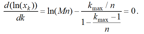
From (16), we have the level number with the most quantity of tree nodes:

(17)

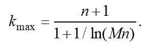
For example, if =15 and =4 the quantity maximum take place on the level number 13. According to formula (14) this maximum is equal to 10¹⁹.